Chapter 4 Methodology

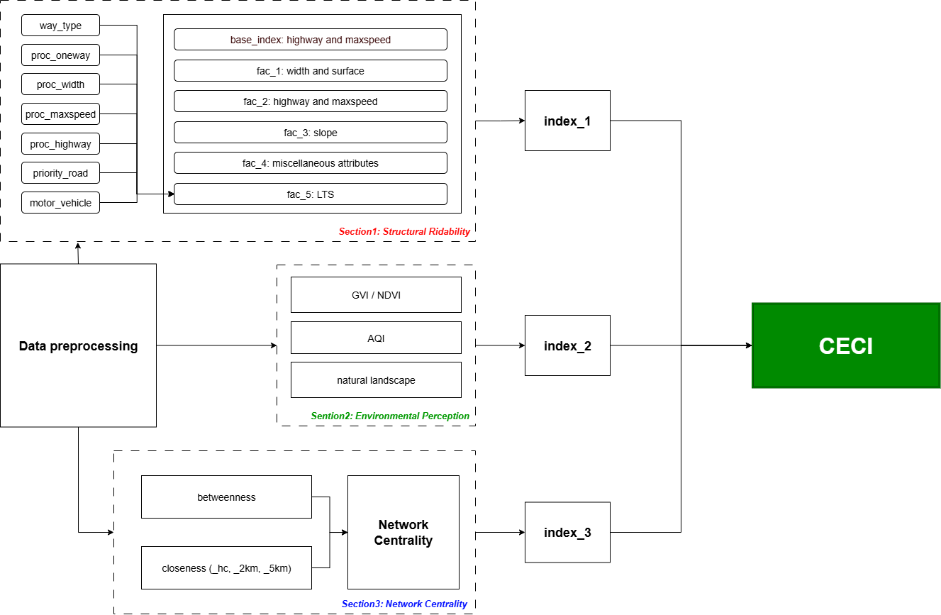
Figure 4.1: Workflow of the Cycling Environment Composite Index (CECI)

Figure 4.1 summarises the end-to-end pipeline for constructing a link-level Cycling Environment Composite Index (CECI) for London. The workflow proceeds through four modules: (1) network acquisition and pre-processing, delivering a cleaned street graph and processed attributes; (2) a structural rideability module that assigns facility- and safety-related factors to each link and produces Index1; (3) an environmental perception module that aggregates greenery, air quality, and natural-landscape proximity into Index2; and (4) a network centrality module that computes graph-theoretic measures and yields Index3. The three sub-indices are winsorised and scaled to a common range and then combined into the CECI under a baseline equal-weights scheme, with predefined alternatives used for robustness. All operations are undertaken in the British National Grid (OSGB36), EPSG:27700. Parameter values and rule tables appear in the Appendix to support reproducibility.

4.1 Network acquisition and pre-processing

Extraction and selection

The base street network is obtained from OpenStreetMap via a two-stage Overpass query. An inclusion-oriented stage captures bicycle-permissible ways across Greater London. A targeted clean removes motorways and ramps, under-construction segments, and links that explicitly prohibit cycling. Direction-dependent rules are implemented for left-hand traffic (right_hand traffic=False).

Topological and geometric cleaning

A light-touch sequence improves graph consistency while preserving OSM geometry. Vertices within 2 m are snapped. Connected components with total length < 100 m are removed. Short dead-end stubs < 20 m are trimmed in three passes. Geometries are clipped to the Greater London boundary. Speed attributes recorded in miles per hour are converted to kilometres per hour (× 1.60934).

Processed fields

Pre-processing yields link-level attributes used downstream: proc_highway, proc_maxspeed, proc_width, proc_oneway, priority_road, motor_vehicle. These standardise tagging and encode London’s traffic handedness.

Normalisation convention

Continuous metrics generated by later modules follow a common scheme: values are winsorised at the 1st and 99th percentiles, then min–max scaled to [0, 1]. Edge betweenness is transformed with log1p before scaling. Normalisation is applied within each sub-index prior to composite scoring.

4.2 Structural rideability (Index1)

4.2.1 Model Introduction

Concept and provenance

The structural module quantifies how road-segment design and operating conditions support everyday cycling. It draws on the open-source OSM Cycling Quality Index developed for Berlin (SupaplexOSM/OSM-Cycling-Quality-Index¹) (SupaplexOSM (2021)), which implements a deterministic, rule-based scoring system over OpenStreetMap data. In that reference model, link-level attributes parsed from OSM—such as functional road class and posted speed, cycleway tags (track/lane/opposite), number of lanes, separation and buffer treatments, surface/smoothness, parking configuration, and basic junction handling—are mapped through factor tables to penalties or bonuses. The Berlin implementation produces a link-level cycling quality score and a separate Level of Traffic Stress (LTS) classification using transparent, auditable rules derived from the above tags and thresholds. The intellectual lineage is acknowledged, and licence and repository details are provided in the Code Availability note.

Adaptations

The adaptation used in this research retains the central idea that compounding frictions are represented by multiplicative factors applied to a base score derived from functional class and speed, while re-specifying inputs and thresholds where necessary for the London context.

During model transfer, several source-model assumptions interact with country-specific OSM tagging practices and data completeness. In particular, the factor slot denoted as fac$_3$ in the reference implementation collapses to a near-constant under London’s OSM coverage (the driving attribute is sparsely or inconsistently recorded, yielding no informative variation at link level). To avoid carrying a non-informative term into the structural score, fac$_3$ is re-specified as a terrain impedance factor derived from segment-level slope.

A further adaptation concerns the role of Level of Traffic Stress (LTS). In the reference framework, Level of Traffic Stress (LTS) and the Cycling Quality Index (CQI) are produced as parallel outputs. To determine whether LTS can be introduced as an additional structural factor within the composite (fac$_5$ in Index1) without undue redundancy, a link-level multicollinearity check was conducted on the set {LTS, fac$_1$, fac$_2$, fac$_4$}. Variables were standardised and analysed using principal components analysis (PCA); segments with incomplete structural attributes were excluded to ensure comparability.

PCA indicates a multi-dimensional structure rather than a single dominant latent factor. The explained-variance ratios are 43.31% (PC1), 25.32% (PC2), 17.18% (PC3), and 14.19% (PC4). Loadings show that LTS aligns chiefly with PC1, while fac$_4$ overwhelmingly defines PC2; fac$_2$ contributes strongly to PC1 and PC3, and fac$_1$ loads on PC1 and PC4. The contrasted signs of LTS and fac$_2$ on PC1, together with the near-orthogonal signal of fac$_4$ on PC2, support the interpretation that these variables capture complementary dimensions rather than a single construct. Summary values are reported in Table 4.1, and the geometry of loadings is visualised in Figure 4.2 (PCA biplot).

Variance inflation factors (VIF) provide a separate, regression-oriented perspective. LTS exhibits low collinearity (VIF = 2.03), with base_index at a moderate level (= 4.63), while fac$_1$ and fac$_2$ show higher mutual dependence (= 27.73 and = 22.36). The low VIF for LTS combined with the PCA results indicates that LTS contributes additional information beyond fac$_1$/fac$_2$/fac$_4$ and can therefore be retained as fac$_5$ in Index1. The pairs plot and correlation matrix provided in the Appendix offer further diagnostic context.

Table 4.1: PCA explained variance and loadings (absolute values).(PC1 = 43.31%, PC2 = 25.32%, PC3 = 17.18%, PC4 = 14.19%)
Variable	PC1	PC2	PC3	PC4
stress_level	0.771	0.04	0.429	0.469
fac1	0.744	0.348	0.198	0.535
fac2	0.724	0.005	0.679	0.124
fac4	0.246	0.944	0.051	0.216

(PC1 = 43.31%, PC2 = 25.32%, PC3 = 17.18%, PC4 = 14.19%)

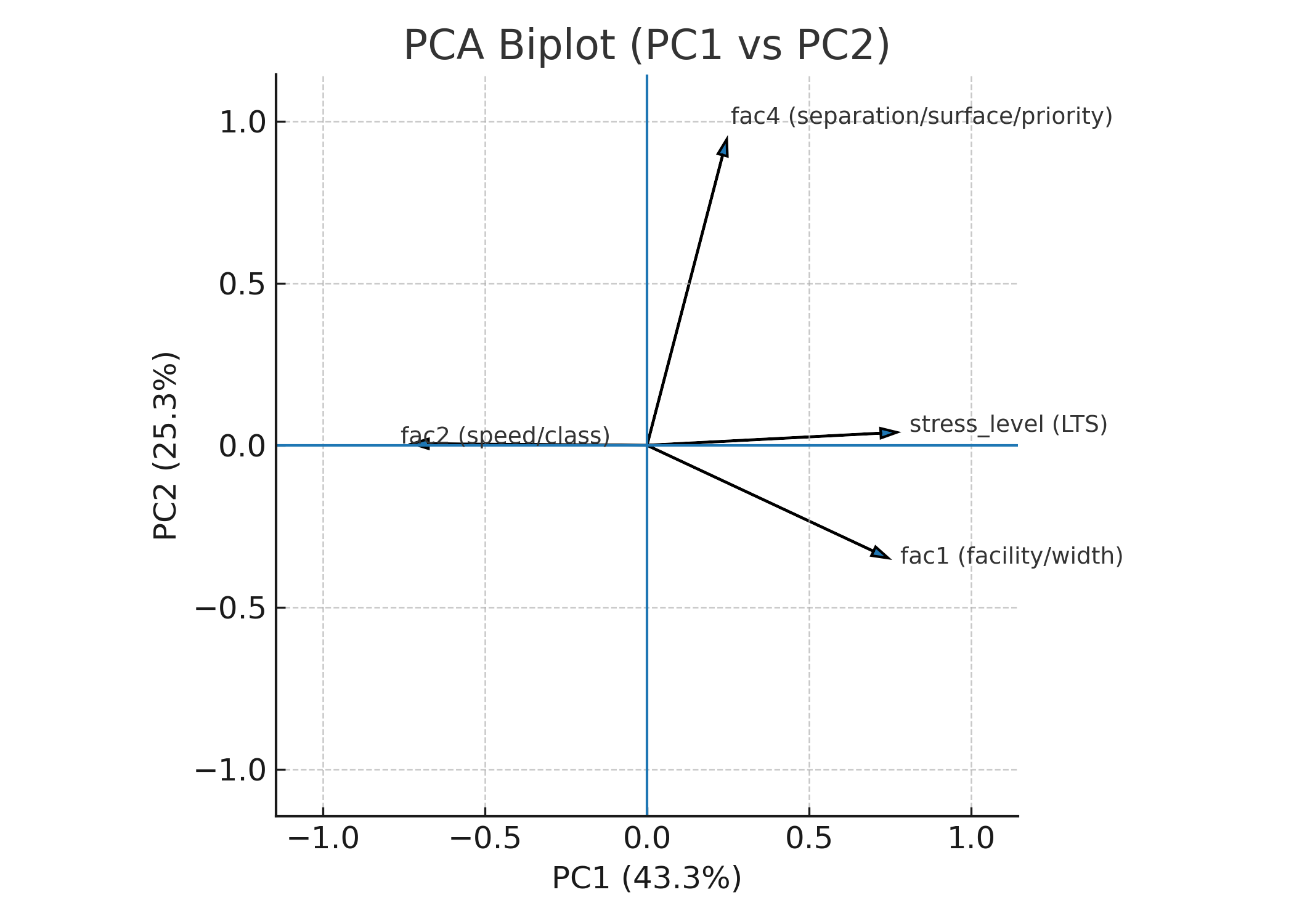
PCA biplot (PC1 vs PC2). Arrows denote variable loadings. LTS (stress level) aligns with PC1; fac$_4$ defines PC2, indicating complementary dimensions.

Figure 4.2: PCA biplot (PC1 vs PC2). Arrows denote variable loadings. LTS (stress level) aligns with PC1; fac$_4$ defines PC2, indicating complementary dimensions.

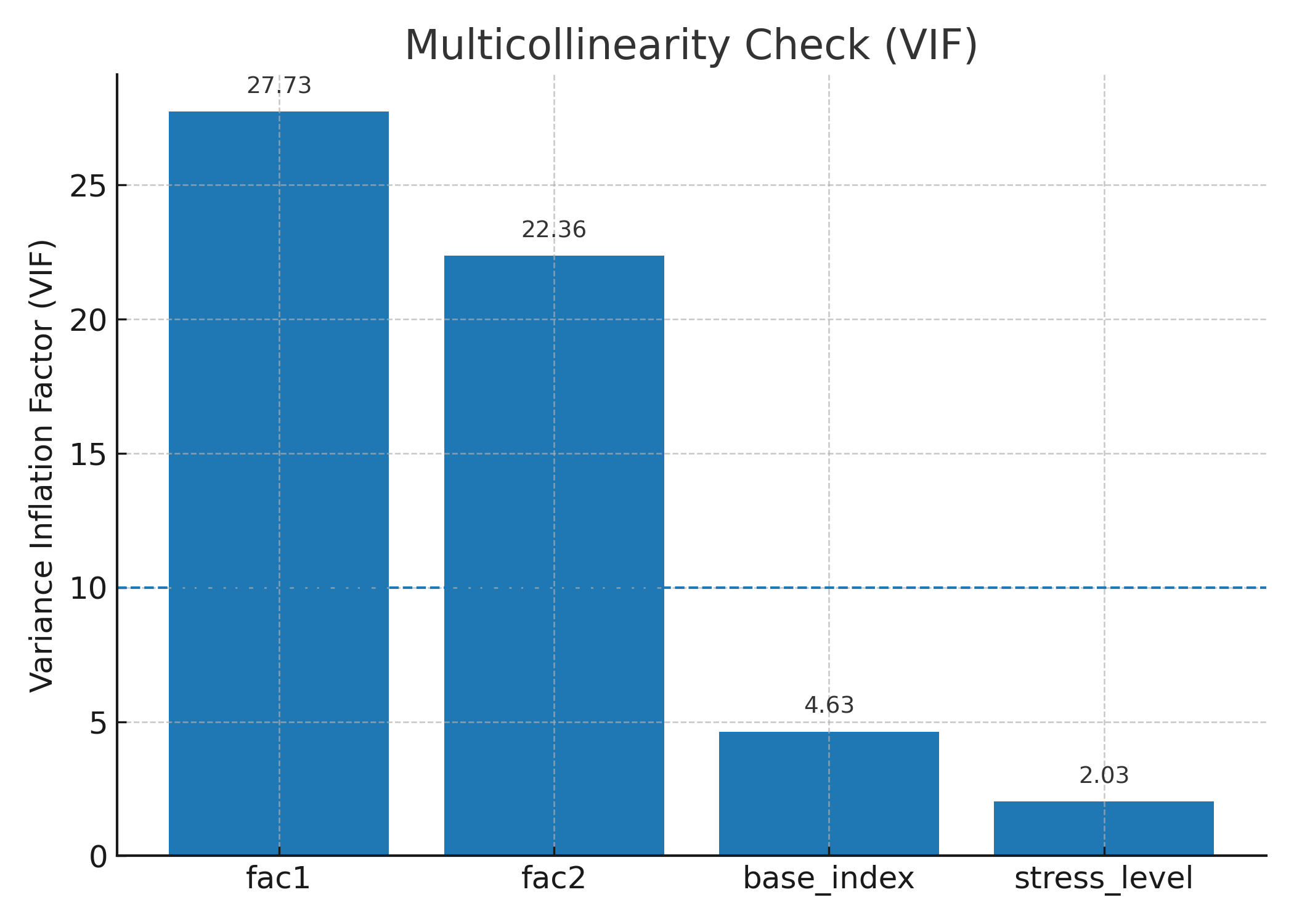
Figure 4.3: Multicollinearity check (VIF). Bars show VIF for the structural variables used in diagnostics. LTS = 2.03, base index = 4.63, fac$_1$ = 27.73, fac$_2$ = 22.36.

These diagnostics justify retaining LTS as an independent factor in Index1, alongside facility/width (fac$_1$), speed/class (fac$_2$), and separation/surface/priority (fac$_4$), within the multiplicative structural specification.

Also, there are some adaptations for left-hand-traffic regime, local speed patterns, and tag conventions to fit in with Great London. The structural specification preserves the core Berlin logic while substituting a slope-based fac$_3$ and justifiably incorporating LTS as fac$_5$, yielding a London-tailored yet methodologically transparent module. Full parameter tables appear in the Appendix.

4.2.2 Data preprocessing

A key element of preprocessing is sidepath identification. Because cycle facilities may be encoded on parallel geometries, a sidepath search prevents under-recognition of protection. Each main link is sampled every 100 m, and a 22 m search radius is used to detect cycle-designated paths. Where a sidepath is found, the main link inherits the relevant facility attributes for scoring, reflecting the facilities realistically available along the corridor.

4.2.3 Engineered attributes and factor mapping

Five categories of factors are computed from processed tags and terrain.

Facility and width (fac$_1$): Functional class together with cycleway:* tags and width inform a factor that rewards physically separated facilities and adequate operating width. Where width is unknown, conservative defaults are used. The mapping distinguishes protected tracks, painted lanes, advisory lanes, and mixed-traffic conditions.
Speed and classification (fac$_2$): Posted speed (proc_maxspeed) and proc_highway class are combined to reflect exposure to motor traffic. Cut-points are calibrated to London’s distribution of speeds and classes and are interpreted under left-hand traffic for oneway segments.
Slope (fac$_3$): Terrain impedance is computed by sampling the 5 × 5 m slope raster along each geometry. Samples are aggregated to a representative segment value (robust statistic as specified in the Appendix) and then mapped to penalty factors. Missing slope receives fac$_3$ = 0.9 as a conservative treatment that avoids unjustified improvement.
Separation, buffer, surface, and priority (fac$_4$): Presence and width of buffers, type of kerb or median separation, parking configuration, surface/smoothness classes, and priority on major roads contribute additional penalties or bonuses. Directionality is evaluated with respect to left-hand traffic (e.g., parking or buffer on the rider’s side). Rule tables provide deterministic mappings from tag combinations to factors.
Level of Traffic Stress (fac$_5$): An LTS class is assigned from the joint configuration of speed, lanes, facility type, and separation (with junction handling consistent with local practice). Classes are translated into factors using the codebook values reported in the Appendix.

4.2.4 Base score and multiplicative formulation

A base score Base(highway, maxspeed) represents the nominal quality of a segment absent additional penalties or bonuses. The structural sub-index is:

\[Index_{1} = Base \times fac_{1} \times fac_{2} \times fac_{3} \times fac_{4} \times fac_{5}\]

followed by linear rescaling to [0, 100]. The multiplicative form ensures that simultaneously adverse attributes (e.g., steep gradient, high speed, lack of separation) reduce scores more than any single attribute alone, reflecting the compounding nature of perceived stress and safety constraints. Conversely, coherent design packages (e.g., protected track with buffer on a low-speed street) achieve proportionally high values.

4.3 Environmental perception (Index2)

4.3.1 Subcomponents and normalisation

The environmental module operationalises three link-level components and combines them after normalisation.

4.3.2 Greenery (GVI)

Link values are obtained by buffering each link midpoint by 30 m (or by regular along-link samples with the same radius) and averaging nearby GVI observations. Instances with no observations inside the buffer are recorded for transparency.

4.3.3 Air quality (NO$_2$)

The gridded NO$_2$ surface (cell size 20 m) is sampled every 10 m along each link and averaged. The normalised value is inverted as (1 − NO$_2$_norm) so that higher values consistently denote better conditions.

4.3.4 Natural-landscape proximity

Polygons representing natural landscapes are dissolved by type to avoid double counting. A multi-ring proximity function is computed around each link using the levels (50 m, 0.1), (40 m, 0.2), (30 m, 0.3), (20 m, 0.5), (10 m, 0.7), (1 m, 1.0); weights increase with proximity.

4.3.5 Sub-index formulation

Considering that NO₂ concentration is more relevant to long-term health than to immediate perceptual experience, and that natural landscapes provide a diffuse but less easily quantifiable contribution to cycling quality, greater weight was assigned to GVI, which directly captures visible greenery and has been shown to strongly shape comfort and safety. Among the three components, GVI was regarded as the most salient and consistently measurable factor influencing perceived cycling quality.

Accordingly, the three components were combined after normalisation to [0, 1] as:

\[Index_{2} = 0.5 \times GVI_{\text{norm}} + 0.3 \times (1 - NO_{2,\text{norm}}) + 0.2 \times Natural_{\text{norm}}\]

then rescaled to [0, 100].

4.4 Network centrality (Index3)

4.4.1 Graph representation

A primal, undirected graph is constructed from the cleaned OSM network. Edge weights equal metric length in metres.

4.4.2 Betweenness

Edge betweenness is estimated using approximate sampling with K = 1200 source pairs. Values are transformed with log1p and min–max scaled.

4.4.3 Range-limited closeness

The National Travel Survey reported that the average cycling trip length in England was approximately 3 miles (around 4.8 km) in 2023 (Department for Transport (2024)). Based on this evidence, closeness centrality was calculated at 2 km and 5 km radii, representing typical short-distance and upper-range commuter cycling trips. Greater weight was assigned to the 2 km radius as local trips dominate everyday cycling patterns, while the 5 km radius captures longer journeys within the average commuting range.

The two scales were combined into a multi-scale composite as:

\[C_{\text{multi}} = 0.6 \times C_{2\text{km}} + 0.4 \times C_{5\text{km}}\]

then scaled to [0, 1].

4.4.4 Sub-index formulation

The centrality sub-index balances through-flow importance and local reachability:

\[Index_{3} = 0.4 \times Betweenness_{\text{norm}} + 0.6 \times C_{\text{multi,norm}}\]

rescaled to [0, 100].

4.5 Composite index, sensitivity, and reporting

4.5.1 Merging and keying

Outputs are joined by a stable key consisting of the OSM id and a hashed edge_uid derived from endpoint coordinates. Geometry is inherited from the structural layer to maintain alignment.

4.5.2 Composite scoring

The Cycling Environment Composite Index (CECI) is the arithmetic mean of the three sub-indices under a baseline equal-weights assumption:

\[CECI = \frac{Index_{1} + Index_{2} + Index_{3}}{3}\]

This choice balances design quality, environmental comfort, and network position at evaluation stage. Length-weighted summaries may subsequently be produced for Borough or MSOA units for descriptive purposes; these aggregations are intentionally separated from model construction.

4.5.3 Sensitivity analysis

To examine robustness to weighting assumptions, three alternative schemes are predefined:

Scheme A (Index1/Index2/Index3): 0.5 / 0.25 / 0.25.
Scheme B (Index1/Index2/Index3): 0.25 / 0.5 / 0.25.
Scheme C (Index1/Index2/Index3): 0.25 / 0.25 / 0.5.

Comparative statistics and maps are reported alongside the baseline.

4.5.4 Quality control and implementation notes

Post-cleaning checks review connectivity and degree distributions. Borough-level sidepath rates are monitored to flag tagging anomalies. Overlay steps (slope, greenery, pollution, natural landscapes) record geometry–attribute counts to confirm coverage before index computation. Normalisation diagnostics document the effect of p1–p99 winsorisation. Processing uses standard Python geospatial libraries (GeoPandas, Shapely, rasterio, OSMnx) and graph tools with fixed random seeds. Parameter files and scripts are available in the project repository.

References

Department for Transport. 2024. “Walking and Cycling Statistics, England: 2023.” Department for Transport. https://www.gov.uk/government/statistics/walking-and-cycling-statistics-england-2023/walking-and-cycling-statistics-england-introduction-and-main-findings-national-travel-survey.

SupaplexOSM. 2021. “OSM Cycling Quality Index.” 2021. https://github.com/SupaplexOSM/OSM-Cycling-Quality-Index.

SupaplexOSM/OSM-Cycling-Quality-Index (GitHub repository, available at https://github.com/SupaplexOSM/OSM-Cycling-Quality-Index), accessed 2025-08-12.↩︎

Developing the Cycling Environmental Composite Index (CECI) to Assess Cycling Friendliness: Evidence from London